Digital Sound Graphs

A digitised sound can be shown on a graph. Time goes on the horizontal axis and amplitude goes on the vertical axis. Amplitude is the height of the sound wave at that moment. The graph lets you see the pattern of the samples stored in the file.

To plot the graph, work through the samples in order. For each sample, use its time as the x-coordinate and its stored amplitude as the y-coordinate, then mark a point. For example, one hit on a drum pad in a music app might give these samples:

Plotting those points gives (0.0, 9), (0.2, 6), (0.4, 3), (0.6, 1) and (0.8, 0). Join each point across to the next sample time at the same amplitude, then up or down to the next sample. This gives a stepped digital waveform, not a smooth curve. Between one sample and the next, the value is shown held at the same level, so the line stays flat and then jumps sharply at the next sample. That is why the graph looks like a set of steps.

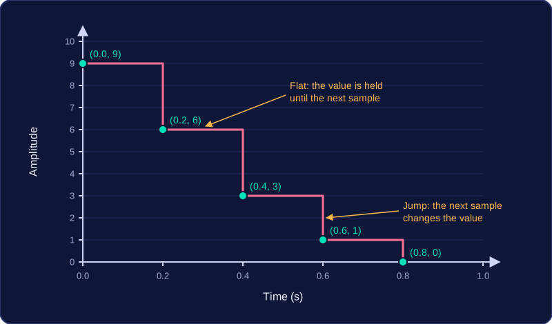
The steps are a picture of the digital data: each flat section shows the amplitude recorded at the last sample, and each jump shows where the next sample changes it.