Algorithms
Search Algorithms

Contents
A search algorithm is a set of steps used to find out whether a particular item is present in a collection of data and, if it is, where it is located. The item you are looking for is called the target.
A search works by comparing the target with items in the list, following the algorithm's steps, until it finds a match or shows that the item is not there. Searching only looks at the data — it never changes it. For example, searching a list of after-school clubs for Chess Club might report that it was found at position 2; if the club is not on the list at all, the search reports that it was not found rather than giving a position.
Successful or unsuccessful
A search that finds the target is successful and reports where the item sits in the list. A search that finishes without a match is unsuccessful and reports that the item is not there. The position is the place in the list, not the value stored at that place.
| Outcome | What it means | What is reported |
|---|---|---|
| Successful | The target was compared with an item and matched | The position of the target in the list |
| Unsuccessful | No comparison matched, so the target is not in the list | That the target was not found |
Two search methods
There are two searching methods you need to know: linear search and binary search. Both can produce a successful or unsuccessful result and both compare a target with items in the data, but their steps are very different.
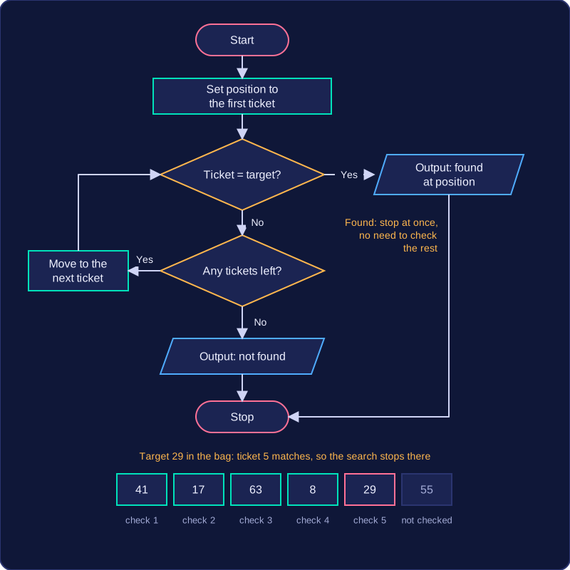
Linear search is the simplest searching algorithm. It finds an item, called the target, by checking the items in a list one after another, starting at the first item.
At each position, the search compares the current item with the target. If they match, it stops immediately and reports that the item has been found, including its position. If the current item does not match, the search moves on to the next item and repeats the comparison. The items are checked in sequence from the start, never in a random order or backwards.
A worked example
Suppose the locker numbers in a corridor are 6, 11, 4, 19 and 23, and you search for 19. The search compares 6 with 19, then 11 with 19, then 4 with 19, then 19 with 19. It stops at the fourth item and reports the match.
| Position | Current item | Match? |
|---|---|---|
| 1 | 6 | No |
| 2 | 11 | No |
| 3 | 4 | No |
| 4 | 19 | Yes: stop |
If the target had been 8, every one of the five items would have been compared before the search reached the end of the list and reported that 19 was not there. The search is only known to be unsuccessful once every item has been checked.
When it suits the job
Linear search does not need the data to be sorted, so it works on ordered or unordered data. It is simple to write, which makes it suitable for small lists, unsorted data and a search that will only be carried out once, where sorting first would add work for little benefit.
Its weakness is speed. If the target is near the end of a large list, or is not there at all, the search may have to check every item, so linear search is slow on large lists.
In Python, a linear search uses one index that starts at the first position and increases by one each time round a loop, comparing each item with the target as it goes.
lockers = [6, 11, 4, 19, 23]
wanted = 19

for position in range(len(lockers)):
    if lockers[position] == wanted:
        print("Found at position", position + 1)
        break
Output:
Found at position 4Tracing a linear search means writing out every comparison the algorithm makes, in order, so that a reader can follow the search from start to finish. The marks come from showing each check you make, not just the final answer.
Laying out each comparison
Linear search always starts at the first item and moves along one item at a time, so your trace must do the same: no jumping ahead, no starting in the middle, no skipping items that look unlikely. A tidy way to write it is one row per comparison, showing the position being checked, the value stored there, and whether it matches.
Take these locker numbers along a corridor: 38, 47, 56, 33, 41, 24. Searching for 33, counting positions from 1:
| Comparison | Position checked | Value stored | Match? |
|---|---|---|---|
| 1 | 1 | 38 | No |
| 2 | 2 | 47 | No |
| 3 | 3 | 56 | No |
| 4 | 4 | 33 | Yes |
The search stops here, after four comparisons, and reports position 4. It does not check 41 or 24, because once a match is found any further comparison is wasted work. Always end a successful trace with that reported position.
A program that prints each comparison as it goes looks like this:
locker_numbers = [38, 47, 56, 33, 41, 24]
wanted_number = 33
place = 0
match_position = -1

while place < len(locker_numbers) and match_position == -1:
    print("Position", place + 1, "holds", locker_numbers[place])
    if locker_numbers[place] == wanted_number:
        match_position = place + 1
    place = place + 1

if match_position == -1:
    print("Not found")
else:
    print("Found at position", match_position)
Output:
Position 1 holds 38
Position 2 holds 47
Position 3 holds 56
Position 4 holds 33
Found at position 4
Position or value?
The position is where an item sits; the value is what is stored there. In the list above, position 4 holds the value 33, so the two numbers are different. Say up front whether you are counting positions from 0 or from 1, then keep to it, since a list counted from 0 would put 33 at position 3. A trace that mixes the two, or that reports the value when asked for a position, is wrong even when the comparisons are right.
When the item is not there
An unsuccessful trace lists every item being compared, one after another, right through to the last one. Only then can you say that the end of the list has been reached and the item is not present. Searching the same list for 50 gives six comparisons, all mismatches, and then the report of not found. That closing statement matters: until every position has been checked, all you know is that the item has not turned up yet, not that it is absent.
In Python, a linear search is built from one loop with a single index that starts at the first position and moves one place at a time, comparing each item with the one you are looking for until it finds a match or reaches the end of the list. That steady, one-place-at-a-time movement is what makes it easy to recognise.
The variables that give it away
A linear search needs an index (often named index) that starts at 0 and has 1 added to it at the end of every pass around the loop, so each item is visited exactly once, in order. Alongside it sit two more variables:
- A found flag, set to
Falsebefore the loop and changed toTrueonly when a match is made, so the code after the loop knows what happened. - A position variable, given the value of the index at the moment of a match, so the search can report where the item was.
Give the position a starting value that could not be a real position, such as -1. The flag, not the position, decides what happens after the loop, so an unsuccessful search reports that the item is missing rather than printing a made-up position.
The loop and its condition
The loop has two jobs: reach every position, and stop early once the item is found. The condition index < len(tickets), together with a check that the flag is still False, does both. The first part keeps the index inside the list, and the second part ends the search the moment a match is made, so later items are never compared.
tickets = [104, 219, 337, 452, 588, 601]
wanted = 452
was_found = False
position = -1
index = 0
while index < len(tickets) and was_found == False:
    if tickets[index] == wanted:
        was_found = True
        position = index
    index = index + 1
if was_found == True:
    print("Ticket", wanted, "was found in slot", position)
else:
    print("Ticket", wanted, "is not in this list")
Output:
Ticket 452 was found in slot 3After the loop, a single if statement tests the flag: True prints the position, and False prints that the item is not in the list.
Getting the loop bounds right
In a list of six items the positions are 0 to 5, so the last valid index is the length minus one and the loop must run while the index is < len(...). Writing <= instead lets the index reach 6, and the next comparison reads past the end of the list.
scores = [14, 27, 31, 46, 58, 69]
wanted = 99
was_found = False
index = 0
while index <= len(scores) and was_found == False:
    if scores[index] == wanted:
        was_found = True
    index = index + 1
print(was_found)
Output:
IndexError: list index out of range (line 6)A binary search finds an item in a sorted list by repeatedly examining the middle item of the part still being searched. The list must be sorted first, or the search may fail.
How it works
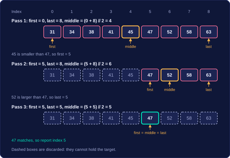
The search area is tracked with a lower bound, an upper bound and a middle position. The middle position is found by integer division of the bounds, which rounds down. If the section has an even number of items, this gives the lower central position.
The middle item is compared with the target. If they match, the search stops and reports the item as found. If the target is smaller or earlier, the middle item and everything after it are discarded, and the upper bound becomes the middle position minus one. If the target is larger or later, the middle item and everything before it are discarded, and the lower bound becomes the middle position plus one. The search repeats on the remaining half.
Worked example
Search for bus route 67 in the sorted route numbers 4, 9, 15, 22, 31, 40, 52, 67, 73, 88, 94, 100.
| Bounds and middle | Value | Action |
|---|---|---|
| 0 to 11, middle 5 | 40 | 67 larger: discard 0 to 5, lower=6 |
| 6 to 11, middle 8 | 73 | 67 smaller: discard 8 to 11, upper=7 |
| 6 to 7, middle 6 | 52 | 67 larger: discard 6, lower=7 |
| 7 to 7, middle 7 | 67 | Match: found at position 7 |
So route 67 was found in four comparisons.
When it is not found
If the lower bound becomes greater than the upper bound, no items remain, so the item is not in the list. For example, searching for route 60 compares 40, then 73, then 52, then 67; after 67, the lower bound 7 is greater than the upper bound 6.
Binary search is faster than linear search on a large sorted list because each comparison discards half the remaining items. It is more complex to write than linear search and needs sorted data: on an unsorted list, discarding half could throw away the target.
To trace a binary search, write down every comparison so someone else can follow the search area shrinking step by step. Each step gives the lower bound, the upper bound and the middle position worked out from them.
Name the item at the middle and say whether it matches the target, is too small or is too large, then which side is discarded and what the new bounds are. If the middle item is too small, the target must lie after it, so the lower bound moves to middle + 1; if it is too large, the upper bound moves to middle – 1. Integer division rounds down, so an even-sized search area uses the left-hand of the two middle items.
A successful trace
Search for 31 in these eight scores at positions 0 to 7: 4, 9, 13, 18, 22, 27, 31, 36.
| Step | Bounds and calculation | Middle item | Result and new bounds |
|---|---|---|---|
| 1 | lower 0, upper 7, middle (0 + 7) // 2 = 3 | 18 | Too small, so 0 to 3 are discarded; lower becomes 4 |
| 2 | lower 4, upper 7, middle (4 + 7) // 2 = 5 | 27 | Too small, so 4 to 5 are discarded; lower becomes 6 |
| 3 | lower 6, upper 6, middle (6 + 6) // 2 = 6 | 31 | Matches, so 31 is found at position 6 and the search stops |
An unsuccessful trace
Now search for 24. Step 1: lower 0, upper 7, middle (0 + 7) // 2 = 3, item 18, too small, so lower becomes 4. Step 2: lower 4, upper 7, middle (4 + 7) // 2 = 5, item 27, too large, so upper becomes 4. Step 3: lower 4, upper 4, middle (4 + 4) // 2 = 4, item 22, too small, so lower becomes 5. The lower bound of 5 is now greater than the upper bound of 4, so the bounds have crossed, no items remain and 24 is not in the list; one mismatch alone only rules out part of the list.
A binary search in Python keeps track of the remaining range of the list using three variables: first, last and middle. first holds the position of the first item in the current range and last holds the position of the last item. middle is the position halfway through that range, calculated from the two bounds:
middle = (first + last) // 2
The // operator is integer division, so the result is rounded down. When the range has an even number of items there are two middle items, and rounding down selects the left-hand one. For example, with first at 0 and last at 7, the calculation gives 3, the left item of the pair at positions 3 and 4.
The loop and its comparisons
The search runs in a loop that continues while the current range still contains items, written in Python as while first <= last. Inside the loop the item at middle is compared with the target:
- If they are equal, the item has been found and
middleis reported as its position. - If the target is smaller,
lastbecomesmiddle - 1, discarding the middle item and everything above it. - If the target is larger,
firstbecomesmiddle + 1, discarding the middle item and everything below it.
Setting a bound to just beyond middle removes the middle item as well as one whole half of the list, so each comparison roughly halves the items left to check.
When first becomes greater than last, the range is empty and the loop finishes, so the search reports that the target is not in the list. The program returns -1 rather than a position, because -1 can never be a real index.
distances = [4, 9, 13, 18, 22, 27, 31, 36, 40]
wanted = 27

def find_position(values, goal):
    first = 0
    last = len(values) - 1
    while first <= last:
        middle = (first + last) // 2
        if values[middle] == goal:
            return middle
        elif values[middle] < goal:
            first = middle + 1
        else:
            last = middle - 1
    return -1

print(find_position(distances, wanted))
Output:
5A search algorithm is used to find a target in a collection of data. Choosing between linear search and binary search depends mainly on whether the data is sorted, how large the list is, and whether you will search it once or many times.
Unsorted data and one-off searches
Linear search works on any list, sorted or not: it starts at the first item and checks items in turn. Binary search only works once the data is sorted into order. If your data is unsorted and you only need to search it once, linear search is usually the sensible choice: sorting first would take time, and that effort only pays off if you plan to make many searches afterwards.
Large sorted lists
If a large list is already sorted, binary search is preferred. It looks at the middle item, compares it with the target, and discards the half that cannot contain the target. Each comparison removes about half of the remaining items, so it needs far fewer comparisons than linear search, which might have to check every item.
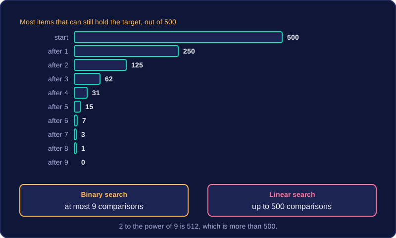
Worked example: in a sorted list of locker numbers from 1 to 320, a binary search for locker 298 compares 160, then 240, 280, 300, 290, 295, 297 and finally 298. That is eight comparisons, while linear search could check 298 lockers. Linear search can be quicker when the target is near the start, because binary search always begins in the middle. If the target is late in the list, linear search has to check almost every item, and if it is absent it checks them all.
Binary search is not always better
Binary search is more complex to write, so it is not automatically the better choice: on a short list, linear search is simpler and finds the item just as quickly. Use linear search for unsorted, small or one-off searches, and binary search for large sorted lists you search repeatedly.